Decision Tree Classifier

The last modifications of this post were around 4 years ago, some information may be outdated!

On this page

What's the idea of Decision Tree Classifier?
Good / Bad of Decision Tree?
When to stop?
When we need to use Decision Tree?
Using Decision Tree Classifier with Scikit-learn
1. Load and create
2. Plot and Save plots
References

What's the idea of Decision Tree Classifier?

The basic intuition behind a decision tree is to map out all possible decision paths in the form of a tree. It can be used for classification and regression (note). In this post, let's try to understand the classifier.

Suppose that we have a dataset $S$ like in the figure below^{[ref, Table 1.2]},

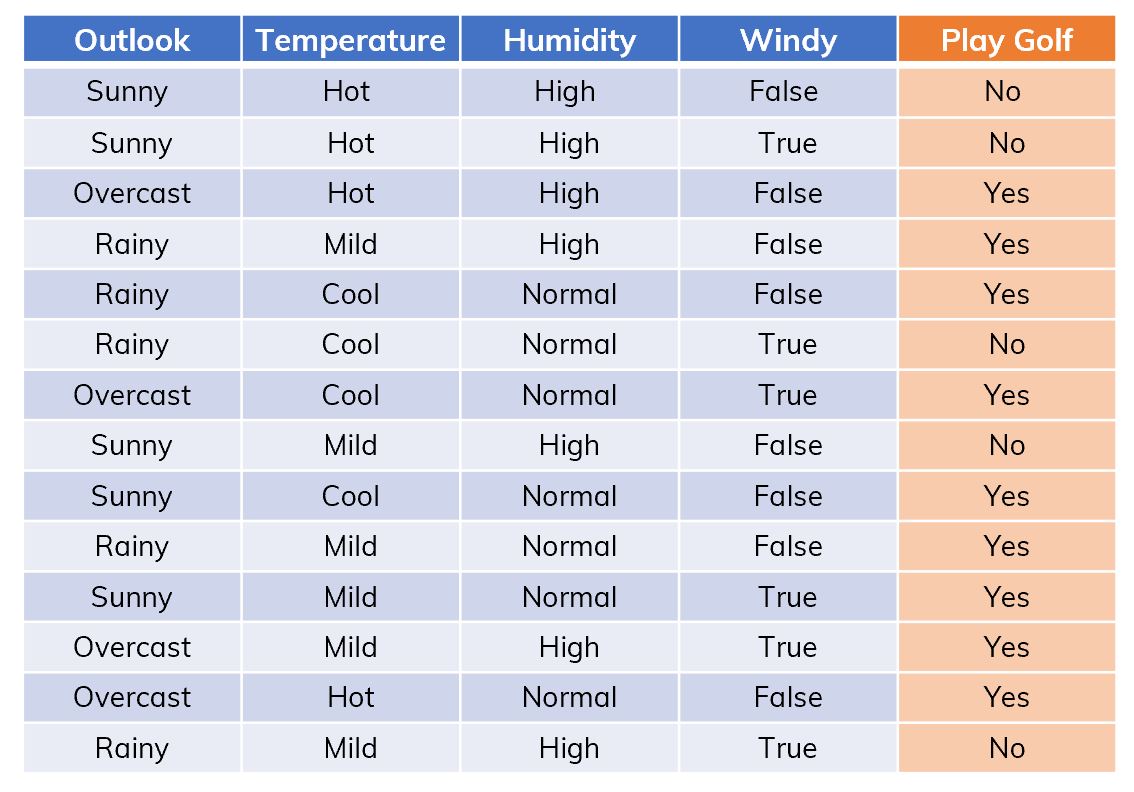
An example of dataset $S$ .

Example of dataset
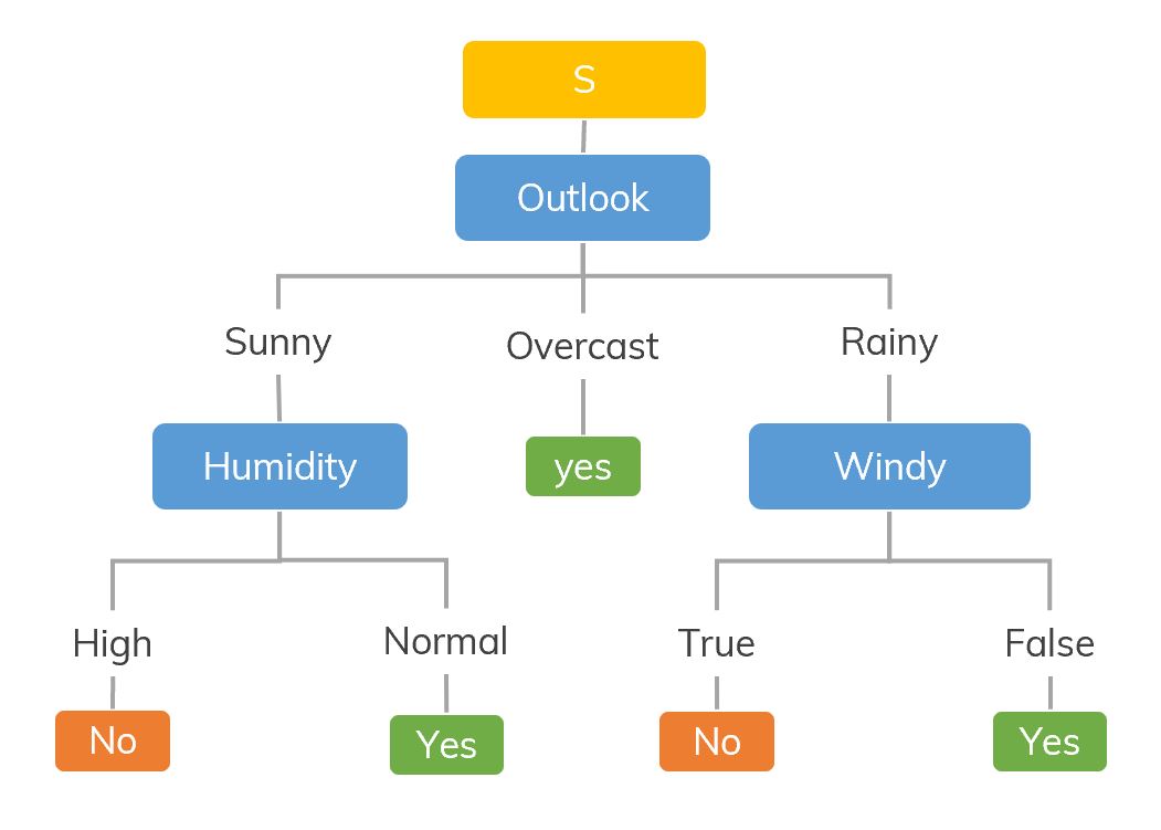
A decision tree we want.

There are many algorithms which can help us make a tree like above, in Machine Learning, we usually use:

ID3 (Iterative Dichotomiser): uses information gain / entropy.
CART (Classification And Regression Tree): uses Gini impurity.

Some basic concepts

Concepts with a tree.

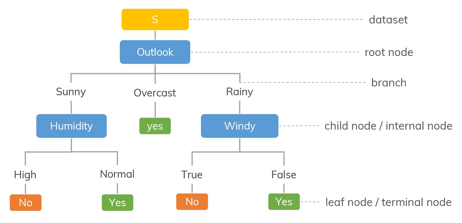
Splitting: It is a process of dividing a node into two or more sub-nodes.
Pruning: When we remove sub-nodes of a decision node, this process is called pruning.
Parent node and Child Node: A node, which is divided into sub-nodes is called parent node of sub-nodes where as sub-nodes are the child of parent node.

ID3 algorithm

ID3 algorithm (TL;DR;)

To check the disorder at current node (let's say $S$ , parent node), we calculate its entropy with,
$H(S) = -\sum_{i=1}^{2} p_{S,i} \log_2 p_{S,i},$
where $i \in$ the number of classes and $p_{S,i}$ is the probability of class $i$ in $S$ .
If entropy at this node is pure (there is only 1 class or the majority is 1 class) or it meets the stopping conditions, we stop splitting at this node. Otherwise, go to the next step.
Calculate the information gain (IG) after splitting node $S$ on each attribute (for example, consider attribute $O$ ). The attribute w.r.t. the biggest IG will be chosen!
$\underbrace{IG(S,O)}_{\text{information gain}} = \underbrace{H(S)}_{\text{entropy before split}} - \underbrace{\sum_j P(O_j | S) \times H(S,O_j)}_{\text{weighted entropy after split}}$
where $j \in$ number of different properties in $O$ and $P(O_j)$ is the propability of property $O_j$ in $O$ .
After splitting, we have new child nodes. Each of them becomes a new parent node in the next step. Go back to step 1.

ID3 algorithm in detail

How we know we can split the dataset $S$ base on the Outlook attribute instead of the others (Temperature, Humidity, Windy)? $\Rightarrow$ We calculate the information gain after splitting $S$ on each attribute. It’s the information which can increase the level of certainty after splitting. The highest one will be chosen (after this section, you will see that the Outlook attribute has the highest information gain).

In order to calculate the information gain, we need "entropy" which is the amount of information disorder or the amount of randomness in the data.

\text{information gain} = \text{entropy before split} - \text{weighted entropy after split}

At the beginning, entropy before split ( $H(S)$ ) shows us the disorder status of the whole dataset $S$ . If $S$ contains only Yes, $S$ has no disorder or it's pure ( $H(S)=0)$ . If the amount of Yes and No in $S$ is equal, $S$ has the highest disorder ( $H(S)=1$ ).

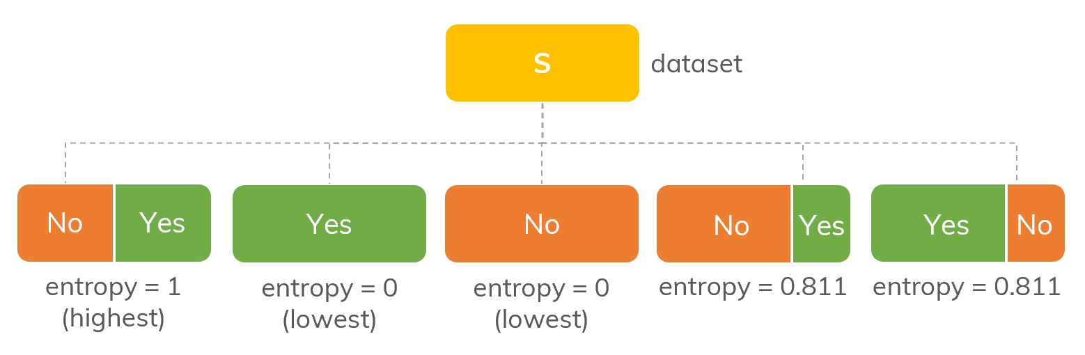
An illustration of entropy with different proportions of Yes/No in $S$ .

At each node, we need to calculate again its entropy (corresponding to the number of Yes and No in this node.). We prefer the lowest entropy, of course! How can we calculate entropy of each node? More specifically, how to calculate $H(S)$ ?

H(S) = -\sum_{i=1}^{2} p_{S,i} \log_2 p_{S,i},

where $i \in$ the number of classes (node $S$ has 2 classes, Yes and No), $p_{S,i}$ is the probability of class $i$ in $S$ .

Graph of H(S) in the case there are 2 classes.
Graph of $H(p)$ in the case of 2 classes. Max is 1.

In this case we use $\log_2$ (binary logarithm) to obtain the maximum $H(S)=1$ and we also use a convention in which $0\times\log_2(0)=0$ . There are other documents using $\log$ (natural logarithm) instead.

On node $S$ , we have,

\begin{aligned} H(S) &= H([9,5]) \\ &= -\frac{9}{14} \times \log_2(\frac{9}{14}) - \frac{5}{14}\times\log_2(\frac{5}{14})\\ &= 0.94. \end{aligned}

We see that, $S$ is not pure but it's also not totally disordered.

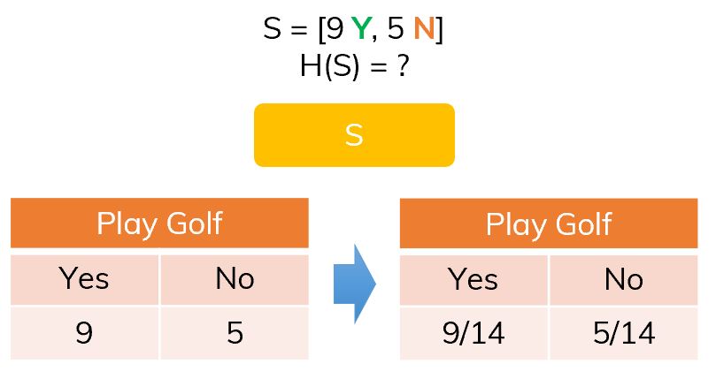
The frequency of classes in S.

Because we are considering to split $S$ on $O$ (Outlook) and $O$ has 3 different properties which are Sunny, Overcast and Rainy. Corresponding to these properties, we have different sizes of Yes/No (Different nodes having different sizes of data but their total is equal to the size of $S$ which is their "parent" node.). That's why we need to calculate the weighted entropy (weighted entropy after split).

\sum_{j=1}^3 P(O_j) \times H(S,O_j),

where $j \in$ number of different properties in $O$ and $P(O_j)$ is the propability of property $O_j$ in $O$ . Therefore, the information gain if split $S$ on $O$ is,

IG(S,O) = H(S) - \sum_{j=1}^3 P(O_j) \times H(S,O_j).

If we split S in O?
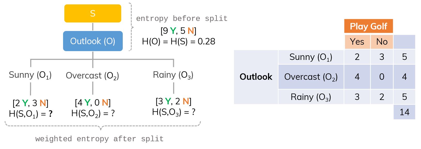
If we split S on Outlook (O), there will be 3 branches.

For example, we consider branch $O_1$ (Sunny), it has $P(O_1)=\frac{5}{14}$ and entropy at this node, $H(S,O_1)$ is calculated as

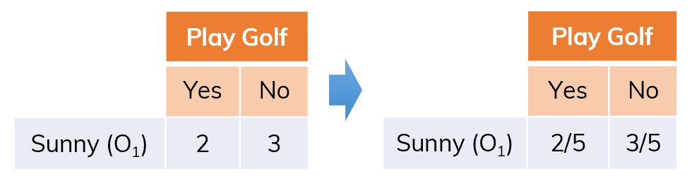
\begin{aligned} H(S,O_1) &= H([2,3]) \\ &= -\frac{2}{5} \times \log_2(\frac{2}{5}) - \frac{3}{5}\times\log_2(\frac{3}{5})\\ &= 0.97. \end{aligned}

Only consider O1
Only consider branch Sunny ( $O_1$ ).

Thus, the information gain after splitting $S$ on $O$ is,

\begin{aligned} IG(S,O) &= H(S) - \sum_{j=1}^3 P(O_j) \times H(S,O_j) \\ &= 0.94 - (\frac{5}{14}\times 0.971 + \frac{4}{14}\times 0 + \frac{5}{14}\times 0.971) \\ &= 0.94 - 0.693 = 0.247. \end{aligned}

With the same method, we can calculate the information gain after splitting $S$ on other attributes (Temperature, Windy, Humidity) and get,

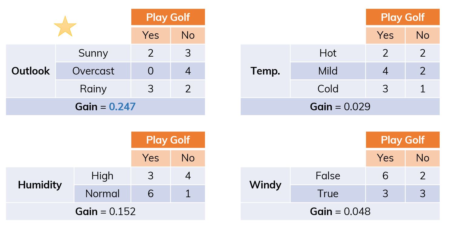
Dataset is split into different ways.

We can see that, the winner is Outlook with the highest information gain. We split $S$ on that attribute first!

Data is split on Outlook.
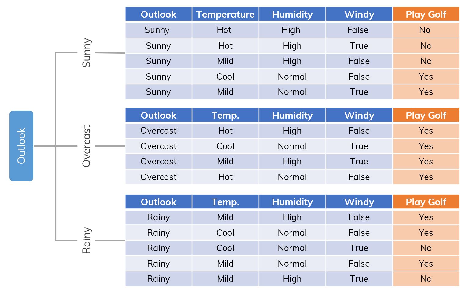
Dataset is split on Outlook.

How about 3 others remaining attributes (Temperature, Humidity, Windy), which one to be chosen next? Especially on branches Suuny and Humidity because on branch Overcast, this node is pure (all are Yes), we don't need to split any more.

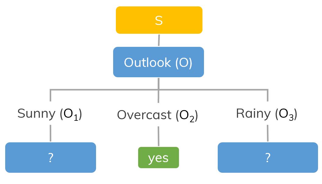
There are remaining Temperature, Humidity, Windy. Which attribute will be chosen next?

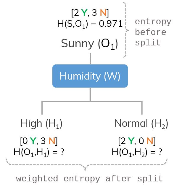
We repeat the steps again, for example, on the branch $O_1$ (Sunny), we calculate IG after splitting $O_1$ on each attribute Temperature (T), Humidity (H) or Windy (W). Other words, we need to calculate $IG(O_1,T)$ , $IG(O_1, H)$ and $IG(O_1, W)$ and then compare them to find the best one. Let's consider $H$ (Humidity) as an example,

\begin{aligned} IG(O_1,H) &= H(O_1) - \sum_{j=1}^2 P(H_j|O_1) \times H(O_1,H_j) \\ &= H(S,O_1) - \frac{3}{5}\times 0 - \frac{2}{5} \times 0 \\ &= 0.971. \end{aligned}

Nodes $W_1$ and $W_2$ are pure, that's why their entropy are $0$ .

Consider branch O1 and attribute W
Consider branch $O_1$ and attribute Windy (W).

Similarly, we calculate $IG(O_1,T)$ , $IG(O_1,H)$ and we see that $IG(O_1,W)$ is the biggest one! So we choose $W$ (Windy) to split at node $O_1$ . On the branch $O_3$ (Rainy), the biggest information gain after splitting is on $H$ (Humidity).

Example of dataset

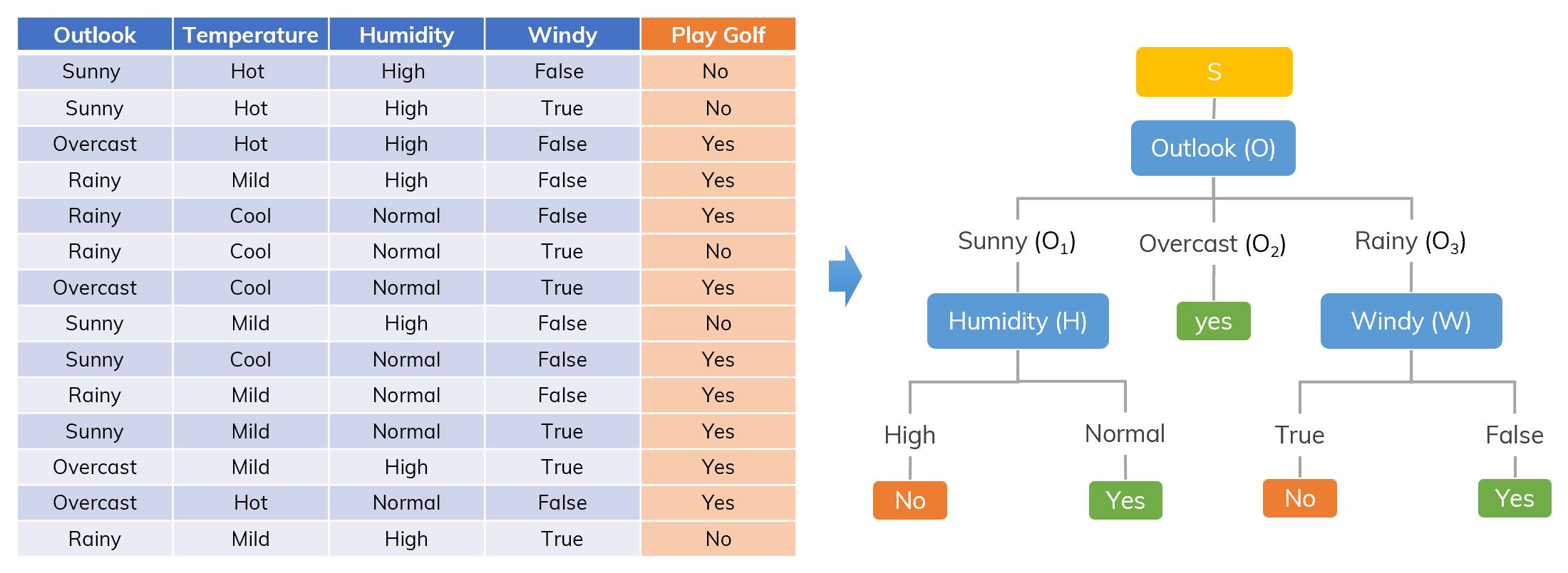
From now, if we have a new input which contains information about Outlook, Temperature, Humidity and Windy, we go from the top of the tree and choose an appropriate branch to get the decision Yes or No.

CART algorithm

CART algorithm (TL;DR;)

The difference between two algorithms is the difference between $H(S)$ and $I_G(S)$ .

To check the disorder at current node (let's say $S$ , parent node), we calculate its Giny Impurity with,
$I_G(S) = \sum_{i=1}^{2} p_{S,i}(1-p_{S,i}),$
where $i \in$ the number of classes in $S$ and $p_{S,i}$ is the probability of class $i$ in $S$ .
If entropy at this node is pure (there is only 1 class or the majority is 1 class) or it meets the stopping conditions, we stop splitting at this node. Otherwise, go to the next step.
Calculate the Gini Gain (GG) after splitting node $S$ on each attribute (for example, consider attribute $O$ ). The attribute w.r.t. the biggest GG will be chosen!
$\underbrace{GG(S,O)}_{\text{gini gain}} = \underbrace{I_G(S)}_{\text{gini impurity before split}} - \underbrace{\sum_j P(O_j | S) \times I_G(S,O_j)}_{\text{weighted gini impurity after split}}$
where $j \in$ number of different properties in $O$ and $P(O_j)$ is the propability of property $O_j$ in $O$ .
After splitting, we have new child nodes. Each of them becomes a new parent node in the next step. Go back to step 1.

CART algorithm in detail

It's quite the same to the ID3 algorithm except a truth that it's based on the definition of Gini impurity instead of Entropy. Gini impurity is a measure of how often a randomly chosen element from the set would be incorrectly labeled if it was randomly labeled according to the distribution of labels in the subset.

At every nonleaf node (which isn't pure), we have to answer a question "Which attribute we should choose to split that node?" We calculate the Gini gain for each split based on the attribute we are going to use. This Gini gain is quite the same as Information gain. The highest one will be chosen.

\text{gini gain} = \text{gini impurity before split} - \text{weighted gini impurity after split}

The Gini Impurity at node $S$ is calculated as,

I_G(S) = \sum_{i=1}^2p_{S,i}(1-p_{S,i}),

where $i\in$ the number of classes in $S$ , $p_{S,i}$ is the probability of class $i$ in $S$ . $I_G=0$ will be the best!

On node $S$ , we have,

\begin{aligned} I_G(S) &= I_G([9,5]) \\ &= \frac{9}{14} \times \frac{5}{14} + \frac{5}{14} \times \frac{9}{14}\\ &= 0.459. \end{aligned}

The frequency of classes in S.

Similarly to the information gain, we can calculate Gini Gain ( $GG$ ) after splitting $S$ on the property $O$ with,

GG(S,O) = I_G(S) - \sum_{j=1}^3 P(O_j) \times I_G(S,O_j),

where $j \in$ number of different properties in $O$ and $P(O_j)$ is the propability of property $O_j$ in $O$ .

If we split S in O?
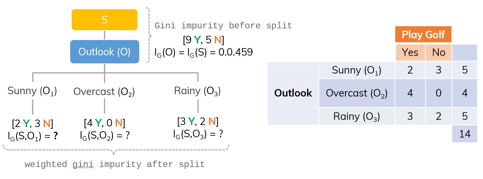
If we split S on Outlook (O), there will be 3 branches.

Apply above equation, we calculate all GG if splitting $S$ on each property and get,

\begin{aligned} GG(S,O) &= I_G([9,5]) - ( \frac{5}{14}\times I_G([2,3]) + \frac{4}{14}\times I_G([4,0]) + \frac{5}{14}\times I_G([3,2])) \\ &= \ldots \end{aligned}

The same for $GG(S,H)$ (Humidity), $GG(S,T)$ (Temperature) and $GG(S,W)$ (Windy). Keep going the same arguments as in the section ID3 in detail, we will get the final tree. The difference between two algorithms is the difference between $H(S)$ and $I_G(S)$ .

Gini Impurity or Entropy?

Some points:^[ref]

Most of the time, they lead to similar trees.^[ref]
Gini impurity is slightly faster.^[ref]
Gini impurity tends to isolate the most frequent class in its own branch of the tree, while entropy tends to produce slightly more balanced trees.

Good / Bad of Decision Tree?

Some highlight advantages of Decision Tree Classifier:^[ref]

Can be used for regression or classification.
Can be displayed graphically.
Highly interpretable.
Can be specified as a series of rules, and more closely approximate human decision-making than other models.
Prediction is fast.
Features don't need scaling.
Automatically learns feature interactions.
Tends to ignore irrelevant features.
Non-parametric (will outperform linear models if relationship between features and response is highly non-linear).

Its disadvantages:

Performance is (generally) not competitive with the best supervised learning methods.
Can easily overfit the training data (tuning is required).
Small variations in the data can result in a completely different tree (high variance).
Recursive binary splitting makes "locally optimal" decisions that may not result in a globally optimal tree.
Doesn't work well with unbalanced or small datasets.

When to stop?

If the number of features are too large, we'll have a very large tree! Even, it easily leads to an overfitting problem. How to avoid them?

Pruning: removing the branches that make use of features having low importance.
Set a minimum number of training input to use on each leaf. If it doesn't satisfy, we remove this leaf. In scikit-learn, use min_samples_split.
Set the maximum depth of the tree. In scikit-learn, use max_depth.

When we need to use Decision Tree?

When explainability between variable is prioritised over accuracy. Otherwise, we tend to use Random Forest.
When the data is more non-parametric in nature.
When we want a simple model.
When entire dataset and features can be used
When we have limited computational power
When we are not worried about accuracy on future datasets.
When we are not worried about accuracy on future datasets.

Using Decision Tree Classifier with Scikit-learn

Load and create

Load the library,

from sklearn.tree import DecisionTreeClassifier

Create a decision tree (other parameters):

# The Gini impurity (default)
clf = DecisionTreeClassifier() # criterion='gini'
# The information gain (ID3)
clf = DecisionTreeClassifier(criterion='entropy')

An example,

from sklearn import tree
X = [[0, 0], [1, 1]]
Y = [0, 1]
clf = tree.DecisionTreeClassifier()
clf = clf.fit(X, Y)
# predict
clf.predict([[2., 2.]])
# probability of each class
clf.predict_proba([[2., 2.]])

array([1])
array([[0., 1.]])

Plot and Save plots

Plot the tree (You may need to install Graphviz first. Don't forget to add its installed folder to $path),

from IPython.display import Image
import pydotplus
dot_data = tree.export_graphviz(clf, out_file=None,
                                rounded=True,
                                filled=True)
graph = pydotplus.graph_from_dot_data(dot_data)
Image(graph.create_png())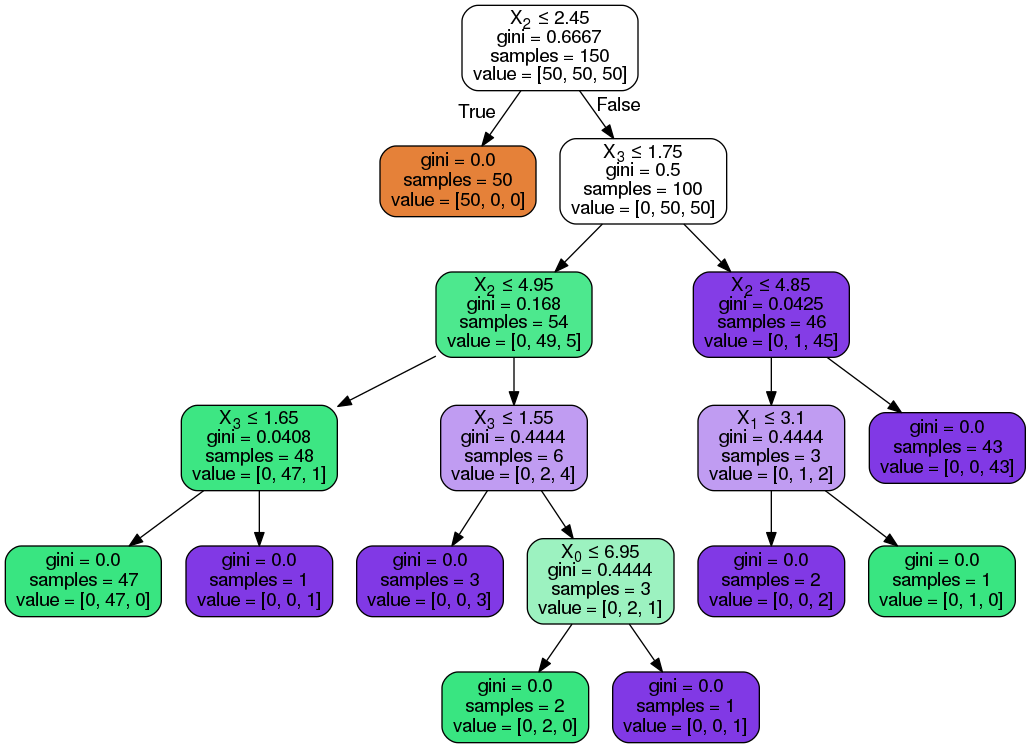

Show figure

Iris tree.

Save the tree (follows the codes in "plot the tree")

graph.write_pdf("tree.pdf")   # to pdf
graph.write_png("thi.png")    # to png

References

Scikit-learn. Decision Tree CLassifier official doc.
Saed Sayad. Decision Tree - Classification.
Tiep Vu. Bài 34: Decision Trees (1): Iterative Dichotomiser 3.
Brian Ambielli. Information Entropy and Information Gain.
Brian Ambielli. Gini Impurity (With Examples).
Aurélien Géron. Hands-on Machine Learning with Scikit-Learn and TensorFlow, chapter 6.