
This is my note for the course (Neural Networks and Deep Learning). The codes in this note are rewritten to be more clear and concise.
👉 Course 1 -- Neural Networks and Deep Learning.
👉 Course 2 -- Improving Deep Neural Networks: Hyperparameter tuning, Regularization and Optimization.
👉 Course 3 -- Structuring Machine Learning Projects.
👉 Course 4 -- Convolutional Neural Networks.
👉 Course 5 -- Sequence Models.
If you want to break into cutting-edge AI, this course will help you do so.
Activation functions
👉 Check Comparison of activation functions on wikipedia.
Why non-linear activation functions in NN Model?
Suppose (linear)
You might not have any hidden layer! Your model is just Logistic Regression, no hidden unit! Just use non-linear activations for hidden layers!
Sigmoid function
- Usually used in the output layer in the binary classification.
- Don't use sigmoid in the hidden layers!
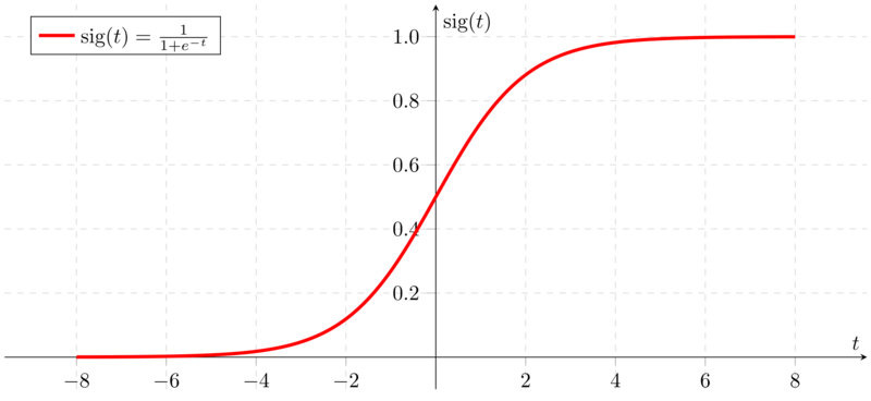
Signmoid function graph on Wikipedia.
import numpy as np
import numpy as np

def sigmoid(z):
    return 1 / (1+np.exp(-z))
def sigmoid_derivative(z):
return sigmoid(z)*(1-sigmoid(z))Softmax function
The output of the softmax function can be used to represent a categorical distribution – that is, a probability distribution over K different possible outcomes.
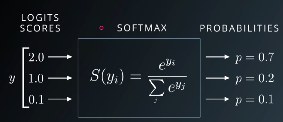
Udacity Deep Learning Slide on Softmax
def softmax(x):
    z_exp = np.exp(z)
    z_sum = np.sum(z_exp, axis=1, keepdims=True)
    return z_exp / z_sum
tanh function (Hyperbolic tangent)
- tanh is better than sigmoid because mean 0 and it centers the data better for the next layer.
- Don't use sigmoid on hidden units except for the output layer because in the case , sigmoid is better than tanh.
def tanh(z):
    return (np.exp(z) - np.exp(-z)) / (np.exp(z) + np.exp(-z))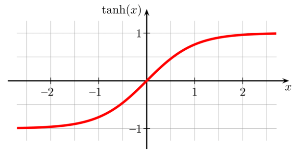
Graph of tanh from analyticsindiamag.
ReLU
- ReLU (Rectified Linear Unit).
- Its derivative is much different from 0 than sigmoid/tanh learn faster!
- If you aren't sure which one to use in the activation, use ReLU!
- Weakness: derivative ~ 0 in the negative side, we use Leaky ReLU instead! However, Leaky ReLU aren't used much in practice!
def relu(z):
    return np.maximum(0, z)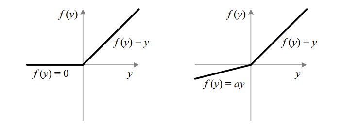
ReLU (left) and Leaky ReLU (right)
Logistic Regression
- Usually used for binary classification (there are only 2 outputs). In the case of multiclass classification, we can use one vs all (couple multiple logistic regression steps).
Gradient Descent
Gradient Descent is an algorithm to minimizing the cose function . It contains 2 steps: Forward Propagation (From to compute the cost ) and Backward Propagation (compute derivaties and optimize the parameters ).
Initialize and then repeat until convergence (: number of training examples, : learning rate, : cost function, : activation function):
The dimension of variables: , , .
Code
def logistic_regression_model(X_train, Y_train, X_test, Y_test,
                              num_iterations = 2000, learning_rate = 0.5):
    m = X_train.shape[1] # number of training examples

    # INITIALIZE w, b
    w = np.zeros((X_train.shape[0], 1))
    b = 0

    # GRADIENT DESCENT
    for i in range(num_iterations):
        # FORWARD PROPAGATION (from x to cost)
        A = sigmoid(np.dot(w.T, X_train) + b)
        cost = -1/m * (np.dot(Y, np.log(A.T))
               + p.dot((1-Y), np.log(1-A.T)))

        # BACKWARD PROPAGATION (find grad)
        dw = 1/m * np.dot(X_train, (A-Y).T)
        db = 1/m * np.sum(A-Y)
        cost = np.squeeze(cost)

        # OPTIMIZE
        w = w - learning_rate*dw
        b = b - learning_rate*db

    # PREDICT (with optimized w, b)
    Y_pred = np.zeros((1,m))
    w = w.reshape(X.shape[0], 1)

    A = sigmoid(np.dot(w.T,X_test) + b)
    Y_pred_test = A > 0.5
Neural Network overview
Notations
- : th training example.
- : number of examples.
- : number of layers.
- : number of features (# nodes in the input).
- : number of nodes in the output layer.
- : number of nodes in the hidden layers.
- : weights for .
- : activation in the input layer.
- : activation in layer , node .
- : activation in layer , example .
- .
Dimensions
- .
- .
- .
- .
L-layer deep neural network
L-layer deep neural network. Image from the course.
- Initialize parameters / Define hyperparameters
- Loop for num_iterations:
- Forward propagation
- Compute cost function
- Backward propagation
- Update parameters (using parameters, and grads from backprop)
- Use trained parameters to predict labels.
Initialize parameters
- In the Logistic Regression, we use for (it's OK because LogR doesn't have hidden layers) but we can't in the NN model!
- If we use , we'll meet the completely symmetric problem. No matter how long you train your NN, hidden units compute exactly the same function No point to having more than 1 hidden unit!
- We add a little bit in and keep in .
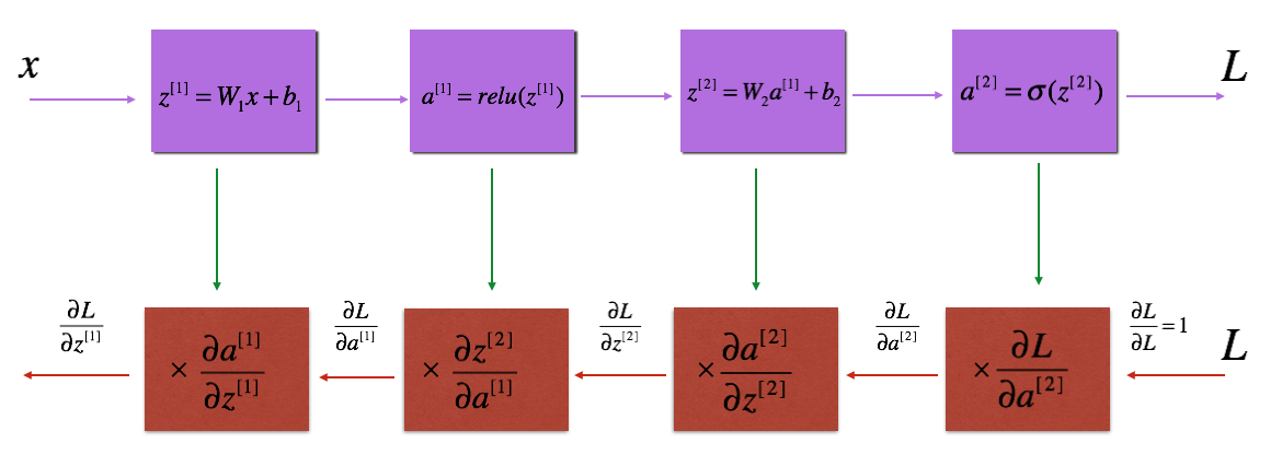
Forward & Backward Propagation
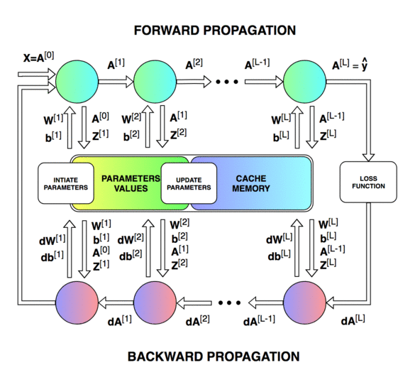
Blocks of forward and backward propagation deep NN. Unknown source.
Blocks of forward and backward propagation deep NN. Image from the course.
Forward Propagation: Loop through number of layers:
- (linear)
- (for , non-linear activations)
- (sigmoid function)
Cost function:
Backward Propagation: Loop through number of layers
- .
- for , non-linear activations:
- .
- .
- .
- .
Update parameters: loop through number of layers (for )
- .
- .
Code
def L_Layer_NN(X, Y, layers_dims, learning_rate=0.0075,
               num_iterations=3000, print_cost=False):
    costs = []
    m = X_train.shape[1] # number of training examples
    L = len(layer_dims)  # number of layers

    # INITIALIZE W, b
    params = {'W':[], 'b':[]}
    for l in range(L):
        params['W'][l] = np.random.randn(layer_dims[l], layer_dims[l-1]) * 0.01
        params['b'][l] = np.zeros((layer_dims[l], 1))

    # GRADIENT DESCENT
    for i in range(0, num_iterations):
        # FORWARD PROPAGATION (Linear -> ReLU x (L-1) -> Linear -> Sigmoid (L))
        A = X
        caches = {'A':[], 'W':[], 'b':[], 'Z':[]}
        for l in range(L):
            caches['A_prev'].append(A)
            # INITIALIZE W, b
            W = params['W'][l]
            b = params['b'][l]
            caches['W'].append(W)
            caches['b'].append(b)
            # RELU X (L-1)
            Z = np.dot(W, A) + b
            if l != L: # hidden layers
                A = relu(Z)
            else: # output layer
                A = sigmoid(Z)
            caches['Z'].append(Z)

        # COST
        cost = -1/m * np.dot(np.log(A), Y.T) - 1/m * np.dot(np.log(1-A), 1-Y.T)

        #FORWARD PROPAGATION (Linear -> ReLU x (L-1) -> Linear -> Sigmoid (L))
        dA = - (np.divide(Y, A) - np.divide(1 - Y, 1 - A))
        grads = {'dW':[], 'db':[]}
        for l in reversed(range(L)):
            cache_Z = caches['Z'][l]
            if l != L-1: # hidden layers
                dZ = np.array(dA, copy=True)
                dZ[Z <= 0] = 0
            else: # output layer
                dZ = dA * sigmoid(cache_Z)*(1-sigmoid(cache_Z))
            cache_A_prev = caches['A_prev'][l]
            dW = 1/m * np.dot(dZ, cache_A_prev.T)
            db = 1/m * np.sum(dZ, axis=1, keepdims=True)
            dA = np.dot(W.T, dZ)
            grads['dW'].append(dW)
            grads['db'].append(db)

        # UPDATE PARAMETERS
        for l in range(L):
            params['W'][l+1] = params['W'][l] - grads['dW'][l]
            params['b'][l+1] = params['b'][l] - grads['db'][l]

    if print_cost and i % 100 == 0:
        print ("Cost after iteration %i: %f" %(i, cost))
    if print_cost and i % 100 == 0:
        costs.append(cost)

    return parameter
Parameters vs Hyperparameters
- Parameters: .
- Hyperparameters:
- Learning rate ().
- Number of iterations (in gradient descent algorithm) (
num_iterations). - Number of layers ().
- Number of nodes in each layer ().
- Choice of activation functions (their form, not their values).
Comments
- Always use vectorized if possible! Especially for number of examples!
- We can't use vectorized for number of layers, we need
for. - Sometimes, functions computed with Deep NN (more layers, fewer nodes in each layer) is better than Shallow (fewer layers, more nodes). E.g. function
XOR. - Deeper layer in the network, more complex features to be determined!
- Applied deep learning is a very empirical process! Best values depend much on data, algorithms, hyperparameters, CPU, GPU,...
- Learning algorithm works sometimes from data, not from your thousands line of codes (surprise!!!)
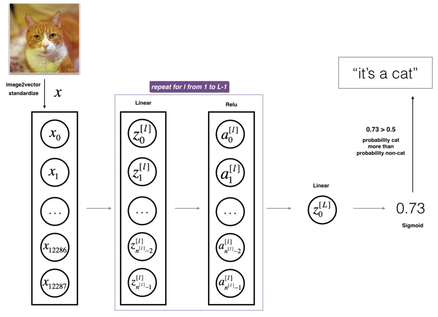
Application: recognize a cat
This section contains an idea, not a complete task!
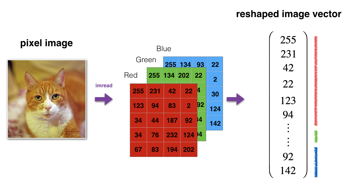
Image to vector conversion. Image from the course.
L-layer deep neural network. Image from the course.
Python tips
○ Reshape quickly from (10,9,9,3) to (9*9*3,10):
X = np.random.rand(10, 9, 9, 3)
X = X.reshape(10,-1).T
○ Don't use loop, use vectorization!
💬 Comments